Chapter 5: How to Read and Interpret EIQ Frequency Analysis
I. Definition and Basics of Frequency Analysis
-
Overview: An analysis method that counts the number of data points (frequency) included in the same value or a specific range (class) to understand the distribution of data.
-
Classes and Intervals: The range used to divide data is called a "Class," and its width is called the "Class Interval." While typically set at equal intervals, EIQ analysis uses unique rules.
II. Uniqueness of Intervals (Ranges) in EIQ Analysis
-
Emphasis on Small-Lot Data: The intervals between 1 and 10 are extremely important; specifically, "Frequency 1" holds significant meaning in the analysis.
-
Adoption of Logarithmic Intervals: As numbers grow larger (e.g., over 100), errors of 10–20% are acceptable. Therefore, using "Logarithmic Intervals" (widening intervals gradually) is more rational than equal ones.
-
Terminology: In EIQ analysis, the term "Range" is used instead of "Interval," based fundamentally on logarithmic frequency distribution.
III. Importance of Frequency 0 (Zero)
-
Application in Inventory Management: Conducting frequency analysis that includes 0 helps identify how many items in stock have "zero shipments" (dead stock).
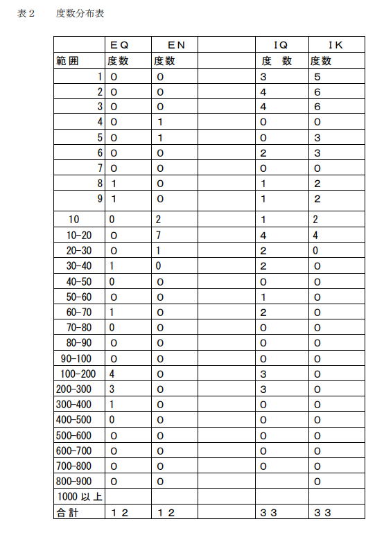
IV. Five Major Frequency Distribution Tables and Histograms
For system planning, frequency analysis is conducted on the following five indicators:
-
EQ Frequency Distribution: Distribution of order quantity per customer per order.
-
EN Frequency Distribution: Distribution of number of order items (hits) per customer per order.
-
IQ Frequency Distribution: Distribution of shipment quantity per product (item).
-
IK Frequency Distribution: Distribution of shipment frequency (order overlap) per product.
-
Q Frequency Distribution: Distribution of order quantity per individual line item on a slip.
V. Analysis Priorities
-
Priority of EN and IK: In system planning, the analysis results of EN (Number of items) and IK (Shipment frequency) are more effective than EQ or IQ, making them the standard starting point.
VI. Simultaneous Presentation of Tables and Histograms
-
Improving Visibility: By attaching histograms alongside specific numerical frequencies and percentages, volume zones can be grasped at a glance.
VII. Interpreting EQ (Order Quantity per Customer)
-
Identifying Large Orders: Identify the ratio of large-scale customers, such as those where orders of 100 cases or more predominate.
-
Operational Decisions: Operational judgments are made, such as determining that Single Picking is suitable if order volumes per customer are large in pallet units.
VIII. Interpreting EN (Items per Customer Order)
-
Trends in Hit Counts: Check whether the number of items ordered is high or low relative to the variety of items in stock.
-
Contextual Inference: High item counts per order with low overall variety is a common characteristic when shipping from food manufacturers to distribution depots.
IX. Ranking via IK (Shipment Frequency per Item)
-
Identifying Best-Sellers: Products with higher order overlap (IK) are the best-selling items.
-
ABC Ranking: This serves as the criteria for classifying products into A (High), B (Medium), and C (Low) based on the frequency of overlap.
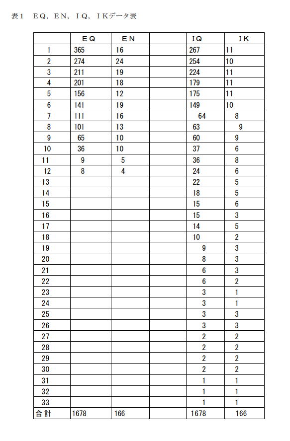
X. Consistency of Total Frequency Values
-
Verification: The sum of frequencies must always match the following values:
-
Total of EQ and EN = Number of order entries (E)
-
Total of IQ and IK = Number of order items (I)
-