Chapter 10: How to Read EIQ Analysis Results (EX0)

I. Interpreting Results for Case Study EX0 (Reference Chapter 15)

• Practical Analysis Explanation: This chapter provides a practical guide on how to read analysis results using the specific case study "EX0," applying the techniques learned so far.
• Integration with Chapter 15: Table and figure numbers cited here correspond to the "EX0" Excel examples in Chapter 15; they should be referenced together.
• Culmination of Learning: The data used for explanations in previous chapters (ABC, Frequency, PCB analysis) are all based on this "EX0".

II. Case Study EX0 Basic Data

This data is based on one day of order slips (or shipping slips), showing the fundamental volume used as the starting point for distribution center planning.

• Number of Orders (E): 12 entries (12 customers), synonymous with shipment count.
• Number of SKUs (I): 33 types, referring to the number of items shipped.
• Total Order Quantity (Q): 1,678 cases, meaning total shipment volume (GQ).
• Total Order Lines (EN): 166 lines (cumulative rows of shipments).
• Inventory Characteristics:
  • Number of Inventory SKUs (ZI): 37 types (calculated from the EIQ table).
  • Inventory Volume (ZQ): Unknown in this specific dataset.

III. EIQ Tables (Table 2, Table 3)

Sorting EIQ Tables and Visualizing Center Characteristics

• Table Composition and Sorting: Table 3 is a version of Table 2 (Basic EIQ Table) sorted by customers with high order quantity (EQ) and items with high shipment volume (IQ).
• Data Concentration Trends: Sorting causes major data with large volumes to gather at the top-left edge, while smaller volumes flow toward the bottom-right.
• Gap between Inventory and Shipments: Checking the bottom row (IQ) of Table 3 reveals that out of 37 inventory SKUs, only 33 actually had orders; the remaining 4 had zero shipment volume.
• Identifying Characteristics: EIQ tables sorted by EQ and IQ are highly effective for visually and quantitatively capturing unique logistics traits, such as bias toward specific customers or products.

IV. EIQNK Table (Table 6)

EIQNK Table Composition, Aggregation, and Consistency

Table 6 (EIQNK Table) adds aggregations for cumulative lines (EN) and overlaps (IK) to the order data, further quantifying logistics characteristics.

• Identifying Maximum Values:
  • By Customer (E6): Customer E6 has the largest order quantity (365 cases) across 16 different items (EN=16).
  • By Item (I5): Item I5 has the largest shipment volume (267 cases), receiving orders from 11 different customers (IK=11).
• Data Aggregation (Right Margin & Bottom Row):
  • Right Margin (Customer Axis): Lists order quantity (EQ) and lines (EN) for each customer, totaling 1,678 cases (GEQ) and 166 lines (GEN).
  • Bottom Row (Item Axis): Lists shipment quantity (IQ) and overlaps (IK) for each item, totaling 1,678 cases (GIQ) and 166 overlaps (GIK).
• Absolute Numerical Consistency:
  • Quantity Invariance: Since order quantity must equal shipment quantity, GEQ = GIQ = 1,678 (GQ).
  • Count Invariance: Since total lines must equal total item overlaps, GEN = GIK = 166.

V. IQ Analysis (Shipment Volume ABC Analysis)

Analyzes bias in shipment volume (IQ) per SKU to inform inventory placement and picking methods. Number of SKUs (I) = 33, Total Shipments (GIQ) = 1,678 cases.

• Grasping Concentration:
  • The top 4 items (10% of the 33 types) account for approx. 55% of total shipments ($I_{10}$ for $IQ_{55}$).
  • The top 8 items (22%) account for approx. 82% of total shipments ($I_{22}$ for $IQ_{82}$).
  • Note: 4 out of 37 types had zero shipments.
• Graph Characteristics: The IQ bar chart (Fig. 3) shows a step-like decrease in approx. 4 stages (ABC), clearly reflecting classification levels. Fig 4 (ΣIQ) shows cumulative values.
• IQ Frequency Distribution (Table 8): There are 6 major items (16%) with shipments of 100 cases or more. Generally, items can be grouped into 3 volume zones: 1–10, 10–70, and 100+.

VI. IK Analysis (Shipment Frequency Analysis)

• IK Frequency Distribution (Table 8): Analyzes how many customers ordered each SKU (hits).
  • Low-Frequency Dispersion: 17 types (over 50%) are ordered by only 1–3 customers.
  • High-Frequency: 6 items (18%) are widely ordered by 10–12 customers.

VII. Order Size and Customer Characteristics

• Definition & Diversity: Order size refers to the quantity ordered by a "specific customer" for a "specific SKU," and these values are highly diverse.
• Grasping via Frequency Distribution: Creating frequency tables for order sizes per customer reveals the actual quantity ranges they typically use.
• Correlation with Customer Scale: Generally, large customers with high total order volume (EQ) have larger order sizes, while smaller customers have smaller ones.
• Mixed Small Orders: Even large customers may have small order sizes (e.g., "1 case") for certain line items; this mix requires attention in planning.

VIII. EN Analysis (Items per Customer Order)

• EN Frequency Analysis (Table 8): Analyzes how many SKUs each customer orders out of the 33 types. 10 customers order 10 or more items, with typical hits ranging from 10 to 20, indicating relatively high variety per order.

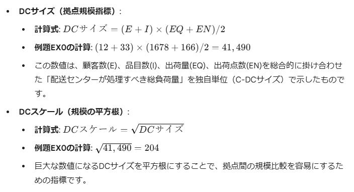
IX. DC Size & DC Scale

The following calculation is used as a quantitative indicator of the distribution center's scale (potential).